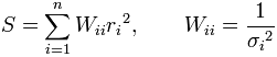
Carl Friedrich Gauss’s method of least squares is a standard approach for sets of equations in which there are more equations than unknowns. Least squares problems fall into two main categories. Linear also know as ordinary least squares and non-linear least squares. The linear least-squares problem pops up in statistical regression analysis and it has a closed-form solution while the non-linear problem has no closed-form solution. Thus the core calculation is similar in both cases.
In a least squares calculation with unit weights, or in linear regression, the variance on the jth parameter, denoted ![]()
is usually estimated with
![]()
Weighted least squares
When that the errors are uncorrelated with each other and with the independent variables and have equal variance, ![]()
is a best linear unbiased estimator (BLUE). If, however, the measurements are uncorrelated but have different uncertainties, a modified approach might be adopted. When a weighted sum of squared residuals is minimized, ![]()
is BLUE if each weight is equal to the reciprocal of the variance of the measurement.
The gradient equations for this sum of squares are
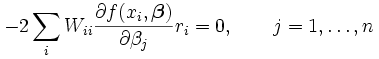
Which, in a linear least squares system give the modified normal equations
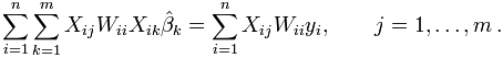
When the observational errors are uncorrelated and the weight matrix, W, is diagonal, these may be written as
![]()
Where
![]()
For non-linear least squares systems a similar argument shows that the normal equations should be modified as follows.
![]()
Important facts about the least squares regression line.
r2 in regression: The coefficient of determination, r2 is the fraction of the variation in the values of y that is explained the least squares regression of y on x.
Calculation of r2 for a simple example:
r2 = (SSM-SSE)/SSM, where
SSM = sum(y-y)2 (Sum of squares about the mean y)
SSM = sum(y-y(hat))2 (Sum of squares of residuals)
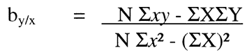
Calculating the regression slope and intercept
The terms in the table are used to derive the straight line formula for regression: y = bx + a, also called the regression equation. The slope or b is calculated from the Y’s associated with particular X’s in the data. The slope coefficient (by/x) equals
THINGS TO NOTE:
· Sum of deviations from mean = 0.
· Sum of residuals = 0.
· r2 > 0 does not mean r > 0. If x and y are negatively associated, then r < 0.
Comments are closed.

![Column Vectors [Mathematics]](https://www.tutebox.com/wp-content/uploads/2010/07/vectors.gif)


Hello, Neat post. There’s an issue along with your web site in web explorer, would check this? IE still is the market leader and a large component to other people will miss your magnificent writing because of this problem.